
Title: Evolution of the Inflaton field
Area:
Country:
Program: Doctors
Available for Download: Yes
View More Student Publications Click here
Abstract
The aim of this thesis is to investigate the evolution of the scalar field by finding the numerical solution and analytical approximation of chaotic inflationary model.
The case of non-minimal coupling is explored by having a non-zero coupling between the inflaton field and gravity. The Higgs inflaton field is considered as the scalar field that led to inflation and the theoretical formulation is described based on the observed data. The analysis of both the numerical and analytical solutions is done using Mathematica.The results of significant experiments will be presented to correlate the theory with the observations. It also shows that the quartic self-coupling can be made large if the coupling of the field to gravity is sufficiently large. The potential is redefined with the modified scalar field after making a conformal transformation from the Jordan frame to the Einstein frame. The transformation is made to reduce the action function without coupling and solved for the scalar field. The results show that the modified scalar field reduces to the original scalar field in the regime of small initial scalar field. Whereas in the case of a large initial field, the modfied field is a logarithmic function of the original field and the resulting Einstein potential is asymptotically flat. The solution to the differential equation in the case of large negative coupling and slow roll inflation conditions, the time evolution of the scalar field is obtained numerically and compared with the corresponding analytical solution.
Acknowledgements
I would like to thank AIU for providing me with a platform for the thesis.
For more information on the AIU's Open Access Initiative, click here.
Chapter 1
Problem statement
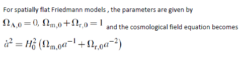
The advantage of the non-minimal inflationary model is that the Higgs boson is the only scalar particle in the Standard Model which is the most probable source of the scalar field driving inflation. The typical model of cosmic inflation includes a scalar field known as the inflaton field to a standard FRW- model. With a suitable assumption of potential, solutions can be obtained to Einstein’s model with homogeneity and isotropy. The solution resembles the slow-roll approximation such that the scalar field which begins with a large, finite value rolls down the potential well. Here the scalar field plays the role of cosmological constant which drives the expansion of the universe. The recent detection of gravitational waves having ripples gives direct proof of inflationary theory and thus settles any doubts regarding it. Evidence suggests that the newer models of inflation with chaotic conditions and eternal inflation have provided the best explanation of the origins of the universe.
Cosmological inflation was proposed by Alan Guth in 1981 and this theory combines general relativity with particle physics. Einstein’s equations give a solution that result in an accelerated expansion of the universe. This places constraints of matter having negative pressure and this is possible with certain models of the scalar fields. The inflationary hypothesis could solve many cosmological problems which include homogeneity, isotropy and the horizon and flatness problems.
Discussion:
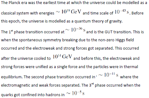
In the inflationary theory, the scalar field inflaton was the cause of rapid expansion and there is a quantized particle corresponding to the field. In the pre-inflationary epoch , the inflaton existed in a higher energy state as mentioned earlier and the phase transitions were caused by quantum fluctuations which led to the release of energy by the inflaton field. The energy was released in the form of radiation and different forms of matter and this led to a repulsive, gravitational force which caused the portion of the current observable universe to expand from 10^-50 meters to 1 meter between 10^-35 and 10^-34 sec.
For the slow-roll approximation to occur, the variation of the energy density with the inflaton field was such that it had a constant high-energy density for high field strengths where it exerted the repulsive force(lasted for about 10^-30). Once the field strength came down to a certain value, there was a decrease in both the energy density and field strength as if it descended the valley, the inflation came to an end. After this, the phase of decelerated expansion began and cooling occurred giving rise to cosmic structures also leading to uniform distribution of matter. The flatness of the current universe is also a consequence of inflation, however, the geometry of the universe prior to inflation is still not confirmed. This implied that the energy density had to be obtained by fine-tuning a parameter very close to 10^-15, such that it produced the right distribution of galaxies with the observed densities.
Research goals and environment
Several space experiments have been conducted to detect the cosmological parameters from the cosmic microwave background, particularly the American Wilkinson Microwave Anisotropy Probe, or WMAP, and the European Planck satellite.
To unravel the characteristics of inflation, the properties of structure formation and anisotropies in temperature were analysed. The correspondence between the scalar perturbations and temperature fluctuations and modes of polarizations were modeled to represent them on large scales. It was observed that scalar perturbations cause E-mode polarizations and tensor perturbations create B-modes. Thus correlation functions are developed to extract information regarding the phenomenon of inflation which is modeled by the theory. WMAP measured the scalar spectral index and tensor to scalar ratio thus obtaining spectral index at ns =0.972 0.013, implying that the universe is either scale invariant or variant and tensor-to-scalar ratio as r < 0.38.
The Planck mission obtained measurements that were more stringent and BICEP2 observed data from a small region of the CMB published in early 2014. They found the fingerprint of primordial tensor perturbations by the presence of B-modes giving r = 0.20 , with r = 0 excluded at 7sigma, or 5.9sigma after subtracting foreground. Therefore, with the data published by planck with r < 0.11, this allows a range of values for epsilon, and exact values for eta and scale dependence of tensor modes. This also allows to explore other methods of Higgs inflation with generalizations to allow for extensions to the scalar field equation and the action function.
Chapter 2
Background information
The typical model of cosmic inflation includes a scalar field known as the inflaton field to a standard FRW- model. With a suitable assumption of potential, solutions can be obtained to Einstein’s model with homogeneity and isotropy. The solution resembles the slow-roll approximation such that the scalar field which begins with a large, finite value rolls down the potential well. Here the scalar field plays the role of cosmological constant which drives the expansion of the universe. The recent detection of gravitational waves having ripples gives direct proof of inflationary theory and thus settles any doubts regarding it. Evidence suggests that the newer models of inflation with chaotic conditions and eternal inflation have provided the best explanation of the origins of the universe.
Cosmological inflation was proposed by Alan Guth in 1981 and this theory combines general relativity with particle physics. Einstein’s equations give a solution that result in an accelerated expansion of the universe. This places constraints of matter having negative pressure and this is possible with certain models of the scalar fields.
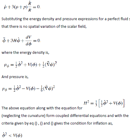
For a perfect fluid, the scalar field would become the cosmological constant ,  if the field has no spatial variation. This is true according to the equation for the enrgy momentum tensor of the fluid and its corresponding
equations for energy density and pressure.
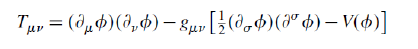
The energy momentum tensor for a scalar field is,
if the field has no spatial variation. This is true according to the equation for the enrgy momentum tensor of the fluid and its corresponding
equations for energy density and pressure.
The energy momentum tensor for a scalar field is,
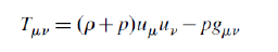
 And for a perfect fluid it is,
 It is thought that inflation occurs between the Planck era and the GUT transition
phase.
On assuming that the universe has followed the radiation-dominated model since
the epoch of inflation which is a
It is thought that inflation occurs between the Planck era and the GUT transition
phase.
On assuming that the universe has followed the radiation-dominated model since
the epoch of inflation which is a
 The present day temperature of the cosmic microwave background is
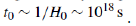
 and the present age of the universe is
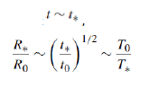
 From the earlier section, the ratio of
 is found to be
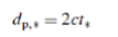
 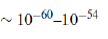 Since the particle horizon at the inflationary epoch is,
 This places constraints on the scalar field potential as the scalar field rolls
between the start and end values(slow roll approximation).
The slow roll approximation states that the evolution of the scalar field with time
must be slow enough to satisfy the condition for inflation. The condition for
inflation is obtained from the equation of motion of the scalar field,
This places constraints on the scalar field potential as the scalar field rolls
between the start and end values(slow roll approximation).
The slow roll approximation states that the evolution of the scalar field with time
must be slow enough to satisfy the condition for inflation. The condition for
inflation is obtained from the equation of motion of the scalar field,
 According to quantum physics, the field is not constant but has random
fluctuations which causes differences in the end times of inflation at different
locations and differences in temperature. The outcomes are not predictable,
unlike the original inflation theory which has predictable outcomes governed by
classical physics. These variations are scale-invariant and hence the magnitudes
are the same on all scales.
According to quantum physics, the field is not constant but has random
fluctuations which causes differences in the end times of inflation at different
locations and differences in temperature. The outcomes are not predictable,
unlike the original inflation theory which has predictable outcomes governed by
classical physics. These variations are scale-invariant and hence the magnitudes
are the same on all scales.
The change in conclusions of inflation began with the realization that inflation is eternal and self-sustaining with irregular fluctuations that re-ignited inflation to produce new regions of matter which non-uniform or warped. When the Universe was very small, these fluctuations are believed to have magnified during the expansion to create galaxies.
The true vacuum state corresponds to the energy density when it rolls down once inflation comes to an end. Energy from the inflaton field is what creates matter according to Einstein’s equation E=mc2
When the early universe is in a state of false vacuum, its negative pressure corresponds to a repulsive gravitational field which drives the region into inflation. This occurs while the density of false vaccum stays constant. This implies that the energy of the expansion keeps increasing which appears to be inconsistent with laws of energy conservation. However, this is resolved since the gravitational energy is descibed as negative by Newton’s theory and during inflation, this energy becomes more negative and balances the positively increasing energy density of matter.
The false vacuum decreases at the end of inflation and the potential energy rolls down releasing it in the form of matter and radiation.
 The horizon problem occurs as a consequence of the deceleration in the
expansion of the universe. The problem is to obtain the reason for the similar
physical characteristics of the vastly separated regions of the universe that had no
causal contact.
A possible solution is to postulate an accelerating phase(known as inflation)
before the deceleration where the remotely separated regions could have had
some causal contact at very early times due to which they shared common
physical characteristics.
The horizon problem occurs as a consequence of the deceleration in the
expansion of the universe. The problem is to obtain the reason for the similar
physical characteristics of the vastly separated regions of the universe that had no
causal contact.
A possible solution is to postulate an accelerating phase(known as inflation)
before the deceleration where the remotely separated regions could have had
some causal contact at very early times due to which they shared common
physical characteristics.
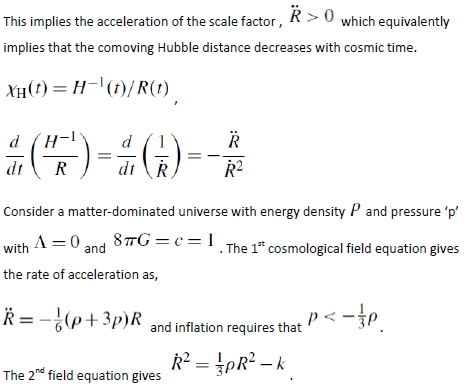 Since the scale factor in an expanding universe must increase such that the
curvature term is negligible for a sufficiently long period of acceleration.
In the early epochs, matter in the form of a scalar field was the physical
mechanism that led to inflation. Quantization of the scalar field describes a
collection of spinless particles.
The universe went through successive stages of phase transitions during its
expansion. The theories that predicted the transitions suggested the existence of
the scalar field.
Depending on the model under consideration,
Since the scale factor in an expanding universe must increase such that the
curvature term is negligible for a sufficiently long period of acceleration.
In the early epochs, matter in the form of a scalar field was the physical
mechanism that led to inflation. Quantization of the scalar field describes a
collection of spinless particles.
The universe went through successive stages of phase transitions during its
expansion. The theories that predicted the transitions suggested the existence of
the scalar field.
Depending on the model under consideration,
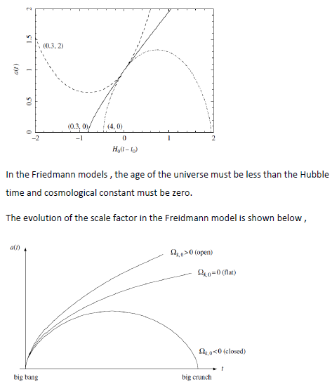
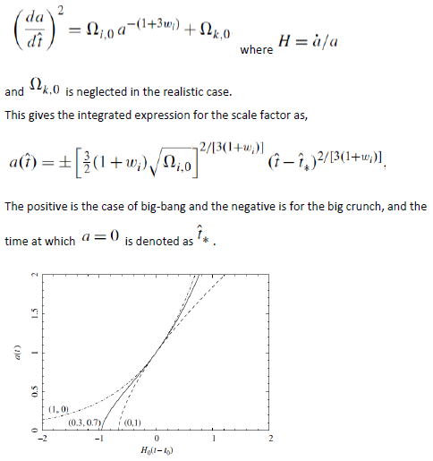 The below graph corresponds to a spatially curved universe with (0.3, 0) for an
open universe and the other two for closed universes.
The below graph corresponds to a spatially curved universe with (0.3, 0) for an
open universe and the other two for closed universes.
 Chapter 3
Thesis statement
The inflationary hypothesis could solve many cosmological problems which include homogeneity, isotropy and the horizon and flatness problems. In this thesis, the dynamics of the scalar field inflaton is modeled to provide solutions with suitable assumptions of the initial conditions and coupling strengths of the scalar field to gravity. The inflation model is based on chaotic inflation where the initial value of the scalar field takes on random values in different regions of the universe. The objective of the thesis will be to explore the evolution of the scalar field by coupling it to the gravitational field to compare the inflaton with the Higgs field of the standard model. This could explain the origins of inflation and whether scalar fields from the Standard model can sufficiently explain inflation. The chaotic mode of inflation is considered with modifications and initial conditions are derived for the perturbations of the scalar field.
Implications: The problem that needs to be explained is the homogeneity of the cosmic microwave background of the universe containing regions vastly separated from each other. The Big Bang theory has predicted anisotropies that are measurable in the sky contrary to the observations. Although cosmic inflation has known to be a solution, it remains to be verified whether the theory is accurate and the causes of inflation. The horizon problem states that the different protions of the universe have not
communicated with each other and yet observations show that they have the same temperature and physical properties. It is believed that radiation cannot travel faster than light to enable heat transfer and thermal equilibrium. Cosmic inflation was a solution since the theory predicted that inflation occurred due to quantum mechanical fluctuations and became the starting point for formation of galaxies that exist currently.
Before the inflation epoch, the universe was as small as 10^-24 cm and all matter and energy were in causal contact. Upon inflation, the connected matter and energy got expanded and travelled futher and further away from each other at the speed of inflationary expansion.The farthest ends are 28 billion light years apart and this raises questions regarding variable speed of light. Although observations of the radiation from the big bang are consistent with inflation theory, more explanations regarding its origins and causes are necessary to resolve the anomalies.
Chapter 4
Methodology
The description of the field theory is given in terms of the Lagrangian formulation
as given by,
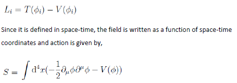 It can be proven that the action is invariant under variation of the field and its
derivatives within the Lagrangian density.
The shape of the scalar field potential determines the evolution of the universe
during the inflationary period. This action is modified by considering it as the
matter component of the Lagrangian and substituted into the Einstein-Hilbert
action. This represents the interaction of the scalar field with the space-time
background and inclusion of a coupling term describes its interaction with gravity.
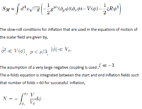
This action for the non-minimally coupled inflaton field is given by,
It can be proven that the action is invariant under variation of the field and its
derivatives within the Lagrangian density.
The shape of the scalar field potential determines the evolution of the universe
during the inflationary period. This action is modified by considering it as the
matter component of the Lagrangian and substituted into the Einstein-Hilbert
action. This represents the interaction of the scalar field with the space-time
background and inclusion of a coupling term describes its interaction with gravity.
This action for the non-minimally coupled inflaton field is given by,
Chapter 5
Strategy and techniques
The chaotic model of inflation was analyzed with the numerical approach and the corresponding analytical approximation. Non-minimal inflation with Higgs inflaton was derived with the slow roll inflation requirements. The effective Higgs potential in the Einstein frame was obtained and the slow parameters where calculated along with the equation for the number of e-folds. The canonical field redefinition was made and the potential expressed in terms of it. With the inflation breakdown condition and number of e-folds for successful inflation, the scalar fields at the end and beginning of inflation were obtained. The numerical solution for the initial scalar field was obtained by including the logarithmic variation and assuming a non-zero value of the end scalar field. The analytical solution was found by neglecting the logarithmic terms and assuming that the end value of the scalar field is non-zero as well as for the case of when it becomes zero. The analytical solution was found for the limits of minimal coupling and for infinitely large coupling and compared with the numerical solution. The effective Einstein potential was considered in the small field and the large field regimes to obtain the relation between the old field and the redefined field. The potential for large fields was considered during the simulation of chaotic inflation with a finite non-minimal coupling constant and quartic potential. The Lagrangian density which includes terms for Einstein-Hilbert action and the coupling terms was considered in the Jordan frame. The redefined field in the Einstein frame was obtained by conformal transformation which redefined the Lagrangian by removing the coupling to gravity. With variational methods, the action was varied with respect to the metric and the scalar fields to obtain the equation of motion for the scalar field. The numerical solution to the resulting equation produced the scalar field as a function of time.
The presentation of data results
Numerical results
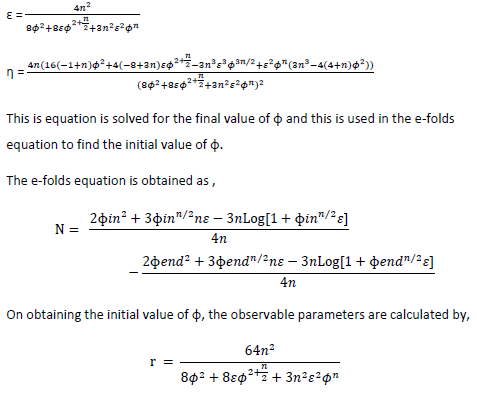
By analysing the behaviour of the slow-roll parameters in limits of ξ-> 0 and ξ -> infinity with the numerical solution,
ϵ = 1 for ε -> 0 gives
Analysis and Results
Numerical Results
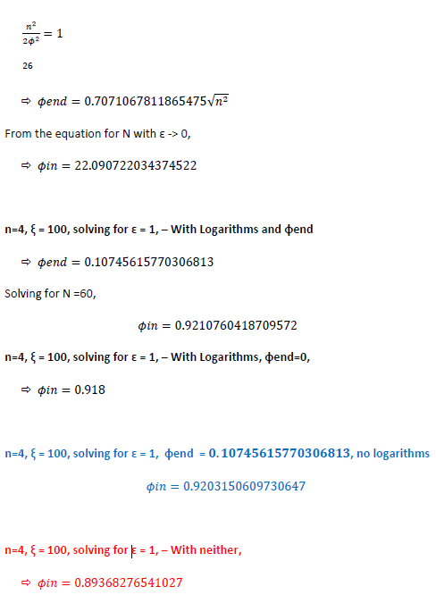
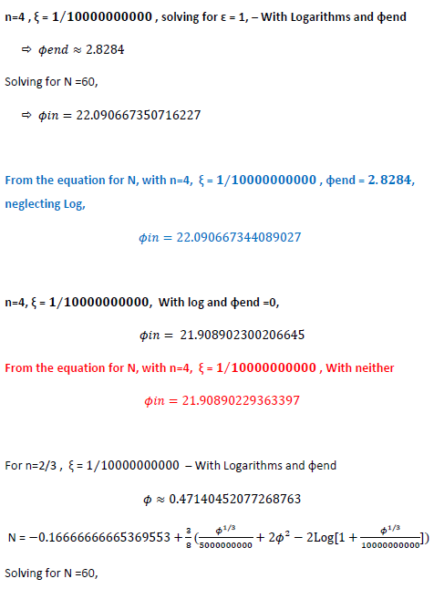
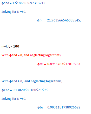
The first aim was to observe the relative errors between the solutions obtained for the scalar field from the e-folds equation. The numerical solutions are compared with the analytical solutions. The solutions are obtained for coupling constant taking on values of 1/1000000000 and 100.
The equation for the slow roll parameter is obtained as,
 Analytical results
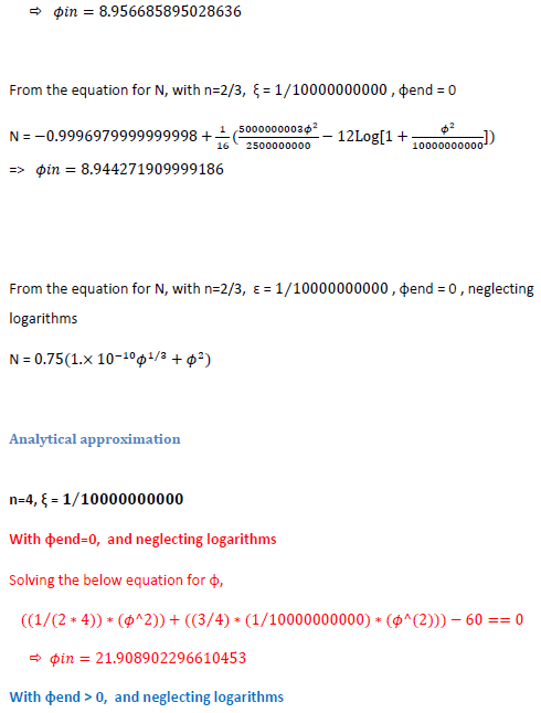
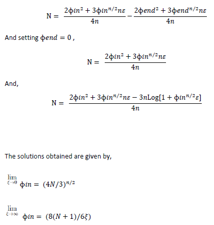
The analytical approximation for ɸin was made by taking the solutions in the limits of ɛ -> 0 and ɛ -> ∞ with ɸend = 0.
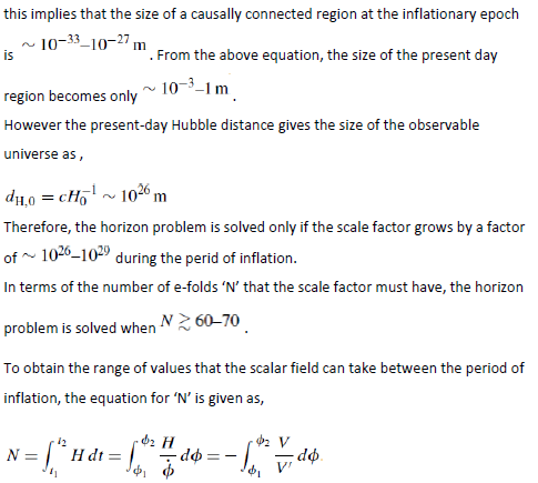
The expression for N neglecting logarithms was obtained as,
Analytical results
The analytical approximation for ɸin was made by taking the solutions in the limits of ɛ -> 0 and ɛ -> ∞ with ɸend = 0.
The expression for N neglecting logarithms was obtained as,
 Questions about alternatives
The Higgs particle has profound implications since all models of inflation are based on a scalar field driven by either its potential energy or kinetic energy. The constraints on the self-coupling constant,λ could be modified such that it takes on an extremely small values in order to reduce the amplitude of the curvature perturbation from the inflaton’s quantum fluctuations. According to the model formulated in this paper, Higgs boson is considered as inflaton only if λ can be sufficiently larger than what is currently.
Therefore a more generalised model that includes extensions in the gravitational theory can be added to the action function, so that the Higgs boson remains the most probable source of inflation in addition to reducing amplitude fluctuations. Thus, a unified treatment of a few different Higgs models can provide the best possible correlation with the current as well as future observations.
Questions about alternatives
The Higgs particle has profound implications since all models of inflation are based on a scalar field driven by either its potential energy or kinetic energy. The constraints on the self-coupling constant,λ could be modified such that it takes on an extremely small values in order to reduce the amplitude of the curvature perturbation from the inflaton’s quantum fluctuations. According to the model formulated in this paper, Higgs boson is considered as inflaton only if λ can be sufficiently larger than what is currently.
Therefore a more generalised model that includes extensions in the gravitational theory can be added to the action function, so that the Higgs boson remains the most probable source of inflation in addition to reducing amplitude fluctuations. Thus, a unified treatment of a few different Higgs models can provide the best possible correlation with the current as well as future observations.
Chapter 6
Conclusions
The difference on neglecting ɸend and the logarithmic terms have been highlighted using the colours which correspond to each sub-case. It has been observed that having only ɸend = 0 does not affect the outcome of the models. Neglecting the logarithms in the chaotic inflation scenario causes the observed parameters to be nearly the same in both the numerical and analytical solutions until a certain value of ξ, after which the deviation from the numerical solution increases and reaches an asymptote. Neglecting both the ɸend and the logarithmic terms causes a minimum deviation for all the lower values of ξ until a certain value, after which the deviation increases to an asymptote with a maximum deviation that is lower than the case of neglecting only logarithms. The evolution of scalar field from the start to the end of inflation has been observed and compared in various cases within the solutions. The alternative approaches to generalizing the higgs inflation model could provide more insights into the properties of observed parameters in future studies.
References
Inflation theory http://universe-review.ca/R02-13-inflation.htm
Philosophy of Cosmology http://www.philosophy-of-cosmology.ox.ac.uk/inflation.html “Non-minimal Higgs Inflation and Frame Dependence in Cosmology”, Steinwachs, Christian Friedrich2014 “The Inflation Debate” , Paul J. Steinhardt “Beyond the Big Bang – Inflation and Early Universe “, Gary Felder
Alan H. Guth, Phys. Rev. D23
A.D. Linde, Phys. Lett. B108, 389 (1982)
J. M. Bardeen, P. J. Steinhardt, and M. S. Turner, Phys. Rev. D28
C. Brans and R. H. Dicke, Phys. Rev. 124, 925 (1961).
D. I. Kaiser, Phys. Rev. D52, 4295 (1995), astro-ph/9408044 Introduction to the Theory of the Early Universe: Hot Big Bang Theory By Dmitriĭ Sergeevich Gorbunov, V. A. Rubakov Quantum Gravitational Correction to Scalar Field Equations During Inflation,by Emre Onur Kahya Modern Cosmology, edited by S Bonometto, V. Gorini, U. Moschella Inflation from Field Theory and String Theory Perspectives, Sebastian Halter Cosmological Inflation and Large-Scale Structure, By Andrew R. Liddle, David H. Lyth Testing Models of Cosmological Inflation, by Christopher Michael Graham,
Towards the theory of reheating after inflation, by Lev Kofman
INFLATION AND BARYOGENESIS THROUGH THE NONMINIMALLY
COUPLED INFLATON FIELD, by Jan WEENINK
Could the Higgs Boson be the Inflaton?, by Michael Atkins
Particle Physics Models of Inflation in Supergravity and Grand Unification,
By Philipp Manuel Kostka
General Relativity: An Introduction for Physicists, by Hobson M, Efstathiou G
Generalized Higgs Inflation models, by Kohei Kamada
Gauge Fields and Inflation, A. Maleknejad, M.M. Sheikh-Jabbari, J. Soda
GREAT EDUCATORS HAVE ALWAYS KNOWN THAT LEARNING IS NOT SOMETHING THAT'S LIMITED TO THE CLASSROOMS, OR THAT SHOULD BE FORCIBLY UNDERTAKEN UNDER THE SUPERVISION OF TEACHERS.
BILL GATES

"BEING DOES NOT MEAN ACCEPTING WHAT ONE IS; IT MEANS CREATING ANOTHER SELF THAT DOES NOT EXIST."
J. CHATEAU